Topic Modeling with R

A topic model is a vision of the world where we are able to decompose written materials into their constituent topics or discourses - if we decide ahead of time how many there will be.

An Introduction to Topic Models#

that link at the end of the video, if you’re interested: http://bit.ly/sw-tm-tour

This course by the way only touches in the lightest manner on the potential for R for doing digital history. Please see Lincoln Mullen’s Computational Historical Thinking with Applications in R for more instruction if you’re interested.

A Walkthrough#

We’re going to use the same data as we did before, but this time, it is organized as a table where each chapbook’s text is one row. There are columns for ‘title’, ‘text’, ‘date’, each separated by a comma, so a bit of the metadata is included. You may download this comma separated, or csv, table from this link.

1. Make a new folder on your computer called chapbooks-r. Put the chapbooks-text.csv inside it.
2. From Anaconda Navigator, open up R Studio. Under ‘File’ select ‘new project’ and then ‘From existing directory.’ In the chooser, select your chapbooks-r folder. Having a ‘project’ in R means that R knows where to look for data, and where to save your work or restore from.
3. Let’s start a new R script. Hit ‘new file’ under ‘file’ (or the button with the green-and-white plus side, top left) and select ‘r script’
4. We need to install some pieces first. In the Console enter these two commands:

install.packages('tidyverse')
install.packages('tidytext')

You’ll only have to do this once. If you get a yellow banner warning across the top of your script screen saying some extra packages weren’t installed and would you like them to be installed, say ‘yes’. If you haven’t encountered the magrittr package, you’ll need to install that too.

5. Now, in our script, let’s begin. We’ll invoke those packages, and load our data up. In this step, we’re also doing a bit of cleaning with a regular expression to remove digits from the text field of our data. You can copy and paste the code below into your R script; run it one line at a time.

# slightly modified version of
# https://tm4ss.github.io/docs/Tutorial_6_Topic_Models.html
# by Andreas Niekler, Gregor Wiedemann

# libraries
library(tidyverse)
library(tidytext)
library(magrittr)

# load, clean, and get data into shape

# cb = chapbooks
cb  <- read_csv("chapbooks-text.csv")

# put the data into a tibble (data structure for tidytext)
# we are also telling R what kind of data is in the 'text',
# 'line', and 'data' columns in our original csv.
# we are also stripping out all the digits from the text column

cb_df <- tibble(id = cb$line, text = (str_remove_all(cb$text, "[0-9]")), date = cb$date)

#turn cb_df into tidy format
# use `View(cb_df)` to see the difference
# from the previous table

tidy_cb <- cb_df %>%
  unnest_tokens(word, text)

# the only time filtering happens
# load up the default list of stop_words that comes
# with the tidyverse

data(stop_words)

# delete stopwords from our data
tidy_cb <- tidy_cb %>%
  anti_join(stop_words)

6. In the console, take a look at how your data has been transformed. Type cb and hit enter - you’ll see a table very much like how your data would look if you opened it in excel. Type cb_df and it’s still table like, but columns and digits are removed. Type tidy_cb and you’ll see it’s a list of words, with metadata indicating which document the word is a part of, and which year the document was written!

Think of it like this: cb_df is a bit like a shopping list:

costco        | eggs, milk, butter, apples
canadian tire | wrench, toolbox, skates

while tidy_cb is a bit like a receipt:

eggs    | costco
milk    | costco
butter  | costco
apples  | costco
wrench  | canadian tire
toolbox | canadian tire
skates  | canadian tire

Transforming your data like this makes it more amenable to text analysis. Let’s continue.

7. We can now transform that list into a matrix, which will enable us to do the topic model. Add, and then run, the following lines to your script:

# this line might take a few moments to run btw
cb_words <- tidy_cb %>%
  count(id, word, sort = TRUE)

# take a look at what you've just done
# by examining the first few lines of `cb_words`

head(cb_words)

# already, you start to get a sense of what's in this dataset...

# turn that into a 'document term matrix'
dtm <- cb_words %>%
  cast_dtm(id, word, n)

8. Now we’ll build the topic model!

require(topicmodels)
# number of topics
K <- 15
# set random number generator seed
# for purposes of reproducibility; this means that any random numbers that get
# generated will also occur in the same sequence if you re-run this code, since
# the random number generator will always start at the same place.

set.seed(9161)

# compute the LDA model, inference via 1000 iterations of Gibbs sampling
topicModel <- LDA(dtm, K, method="Gibbs", control=list(iter = 500, verbose = 25))

Computers sometimes need to use random numbers in their calculations. By using set.seed, we enable the machine to generate the same sequence of random numbers every time we do these calculations. The effect is that my results and your results will look the same. If you remove the seed, your results will differ from mine in slightly different, minor, ways. It is, after all, a probabilistic process.

Here we’re building a model with 15 topics; we run it for 500 iterations. You can tweak those variables if, after examining the results, you find that the model captures too much (or not enough) variability. The topicModel command takes a bit of time to run, even at just 500 iterations. The higher-end computer you have, the quicker this will run.

9. Now, remember that every document will be composed of all 15 topics, just in different proportions; similarly, every topic has every word, but again, in different proportions. So we’ll rearrange things just so that, say, we get the top 5 terms per topic; these 5 words will give us a sense of what the topic is about. Do you spot where you might change that to say 10 terms?

# have a look a some of the results (posterior distributions)
tmResult <- posterior(topicModel)

# format of the resulting object
attributes(tmResult)

# lengthOfVocab
ncol(dtm)

# topics are probability distributions over the entire vocabulary
beta <- tmResult$terms   # get beta from results
dim(beta)

# for every document we have a probability distribution of its contained topics
theta <- tmResult$topics
dim(theta)

top5termsPerTopic <- terms(topicModel, 5)
topicNames <- apply(top5termsPerTopic, 2, paste, collapse=" ")
topicNames

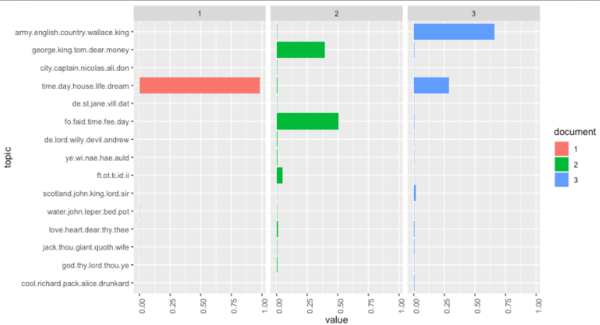
10. Now comes the fun part - visualization of the patterns!

# load libraries for visualization
library("reshape2")
library("ggplot2")

# select some documents for the purposes of
# sample visualizations
# here, the 2nd, 100th, and 200th document
# in our corpus

exampleIds <- c(2, 100, 200)

N <- length(exampleIds)
# get topic proportions form example documents
topicProportionExamples <- theta[exampleIds,]
colnames(topicProportionExamples) <- topicNames

# put the data into a dataframe just for our visualization
vizDataFrame <- melt(cbind(data.frame(topicProportionExamples), document = factor(1:N)), variable.name = "topic", id.vars = "document")

# specify the geometry, aesthetics, and data for a plot
ggplot(data = vizDataFrame, aes(topic, value, fill = document), ylab = "proportion") +
  geom_bar(stat="identity") +
  theme(axis.text.x = element_text(angle = 90, hjust = 1)) +
  coord_flip() +
  facet_wrap(~ document, ncol = N)

11. Finally, let’s look at our topic model over time, which is why you’re all here, right?

#topics over time
# append decade information for aggregation
cb$decade <- paste0(substr(cb$date, 0, 3), "0")
# get mean topic proportions per decade
topic_proportion_per_decade <- aggregate(theta, by = list(decade = cb$decade), mean)
# set topic names to aggregated columns
colnames(topic_proportion_per_decade)[2:(K+1)] <- topicNames

# reshape data frame, for when I get the topics over time thing sorted
vizDataFrame <- melt(topic_proportion_per_decade, id.vars = "decade")

# plot topic proportions per deacde as bar plot
require(pals)
ggplot(vizDataFrame, aes(x=decade, y=value, fill=variable)) +
  geom_bar(stat = "identity") + ylab("proportion") +
  scale_fill_manual(values = paste0(alphabet(20), "FF"), name = "decade") +
  theme(axis.text.x = element_text(angle = 90, hjust = 1))

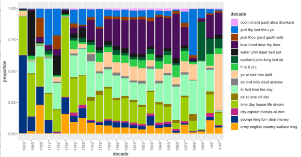
Interesting how stories about the army and the English seem to decrease over time in the 18th century… perhaps that’s meaningful? Go back and re-run your script from the point where you selected 15 topic models. Try more topic models. Try fewer. Do you spot any interesting patterns?

Save your script as tm.R. Put it in your github repo. Save screenshots of your findings, and make notes of your observations. These can be shared in your weekly work too - make sure the image file and your notes.md file are in the same repository, then you can insert an image like this:

![description of image](filename.jpg)

or filename.png etc.

Now, there’s a lot in this code that is impenetrable to you right now. But frankly, there is a lot that goes on under the hood for any tool, but it is hidden behind a user interface. At least here, you can see what it is that you do not yet understand. One of the attractions of doing this kind of work in R and R Studio is that these scripts are reusable, shareable, and citeable. A script like this might accompany a journal article, allowing the reviewers and the readers alike to experiment and see if the author’s conclusions are warranted. Alternatively, you could replicate the study on a different body of evidence, provided that you arranged your data in the same way our original source tables were arranged.

Communicating the process, the meat-grinding, of your research this way leads to better research. And it’s a helluva lot easier to point to a script than say ‘now click this… then this… then if you’re using this version, there should be a drop down over here, otherwise it’ll be… now click the thing that looks like…’

Chantal Brousseau has an R-powered notebook about interactive topic models online at Binder if you’d like to explore some more. Depending on when someone last visited that link (thus triggering the website to build the virtual computer to run the notebook) it might take several minutes to load.